- **前提已知**:事件平均发生率为λ
- **推导结果**:在给定时间内发生k次的概率是多少
泊松分布是 [二项分布](二项分布.md) 的极限形式
<!-- more -->
用一个 " 栗子 " 讲清楚泊松分布 - 梁唐的文章 - 知乎
https://zhuanlan.zhihu.com/p/139114702
是的,泊松分布可以看作是二项分布在某些条件下的极限情况。具体来说,当二项分布的试验次数 (n) 趋向于无穷大,同时成功的概率 (p) 趋向于零,但 (np)(即期望值)保持恒定时,二项分布将趋近于泊松分布。
# 泊松分布
泊松分布的**本质还是二项分布**,泊松分布只是用来简化二项分布计算的。就是二项分布公式的函数图像在 index 数量无穷大处的一个等价的函数表达式
# HashMap 的链表转红黑树阈值
```java
/*
* Implementation notes.
*
* This map usually acts as a binned (bucketed) hash table, but
* when bins get too large, they are transformed into bins of
* TreeNodes, each structured similarly to those in
* java.util.TreeMap. Most methods try to use normal bins, but
* relay to TreeNode methods when applicable (simply by checking
* instanceof a node). Bins of TreeNodes may be traversed and
* used like any others, but additionally support faster lookup
* when overpopulated. However, since the vast majority of bins in
* normal use are not overpopulated, checking for existence of
* tree bins may be delayed in the course of table methods.
*
* Tree bins (i.e., bins whose elements are all TreeNodes) are
* ordered primarily by hashCode, but in the case of ties, if two
* elements are of the same "class C implements Comparable<C>",
* type then their compareTo method is used for ordering. (We
* conservatively check generic types via reflection to validate
* this -- see method comparableClassFor). The added complexity
* of tree bins is worthwhile in providing worst-case O(log n)
* operations when keys either have distinct hashes or are
* orderable, Thus, performance degrades gracefully under
* accidental or malicious usages in which hashCode() methods
* return values that are poorly distributed, as well as those in
* which many keys share a hashCode, so long as they are also
* Comparable. (If neither of these apply, we may waste about a
* factor of two in time and space compared to taking no
* precautions. But the only known cases stem from poor user
* programming practices that are already so slow that this makes
* little difference.)
*
* Because TreeNodes are about twice the size of regular nodes, we
* use them only when bins contain enough nodes to warrant use
* (see TREEIFY_THRESHOLD). And when they become too small (due to
* removal or resizing) they are converted back to plain bins. In
* usages with well-distributed user hashCodes, tree bins are
* rarely used. Ideally, under random hashCodes, the frequency of
* nodes in bins follows a Poisson distribution
* (http://en.wikipedia.org/wiki/Poisson_distribution) with a
* parameter of about 0.5 on average for the default resizing
* threshold of 0.75, although with a large variance because of
* resizing granularity. Ignoring variance, the expected
* occurrences of list size k are (exp(-0.5) * pow(0.5, k) /
* factorial(k)). The first values are:
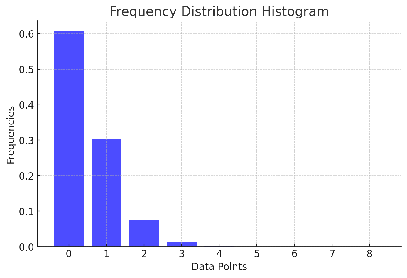
*
* 0: 0.60653066
* 1: 0.30326533
* 2: 0.07581633
* 3: 0.01263606
* 4: 0.00157952
* 5: 0.00015795
* 6: 0.00001316
* 7: 0.00000094
* 8: 0.00000006
* more: less than 1 in ten million
*
* The root of a tree bin is normally its first node. However,
* sometimes (currently only upon Iterator.remove), the root might
* be elsewhere, but can be recovered following parent links
* (method TreeNode.root()).
*
* All applicable internal methods accept a hash code as an
* argument (as normally supplied from a public method), allowing
* them to call each other without recomputing user hashCodes.
* Most internal methods also accept a "tab" argument, that is
* normally the current table, but may be a new or old one when
* resizing or converting.
*
* When bin lists are treeified, split, or untreeified, we keep
* them in the same relative access/traversal order (i.e., field
* Node.next) to better preserve locality, and to slightly
* simplify handling of splits and traversals that invoke
* iterator.remove. When using comparators on insertion, to keep a
* total ordering (or as close as is required here) across
* rebalancings, we compare classes and identityHashCodes as
* tie-breakers.
*
* The use and transitions among plain vs tree modes is
* complicated by the existence of subclass LinkedHashMap. See
* below for hook methods defined to be invoked upon insertion,
* removal and access that allow LinkedHashMap internals to
* otherwise remain independent of these mechanics. (This also
* requires that a map instance be passed to some utility methods
* that may create new nodes.)
*
* The concurrent-programming-like SSA-based coding style helps
* avoid aliasing errors amid all of the twisty pointer operations.
*/```
更详细的解释:
二项分布描述了在 (n) 次独立试验中,成功次数 (k) 的概率,每次试验成功的概率为 (p)。其概率质量函数为:
P(X = k) = \binom{n}{k} p^k (1-p)^{n-k}
其中,(\binom{n}{k}) 是组合数,表示从 (n) 次试验中选出 (k) 次成功的方法数。
当 (n) 很大且 (p) 很小时,计算二项分布的概率会变得复杂。在这种情况下,我们可以通过以下步骤将二项分布转化为泊松分布:
1. 设定期望值:令 ( \lambda = np ),并保持 ( \lambda ) 为常数。
2. 调整参数:随着 ( n ) 趋向于无穷大, ( p ) 趋向于零,同时保证 ( \lambda ) 不变。
在这种条件下,二项分布的概率质量函数可以近似为泊松分布的概率质量函数:
P(X = k) \approx \frac{\lambda^k e^{-\lambda}}{k!}
这是因为当 (n) 趋向于无穷大且 p 很小时,组合数和幂函数的乘积可以近似为泊松分布的形式。
举例说明:
假设我们有一个事件,平均每分钟发生 5 次(即 \lambda = 5)。如果我们把这 1 分钟分成非常多的子间隔(例如每秒),那么每个子间隔内事件发生的概率就会非常小,但总体的期望值还是 5 次。这种情况下,我们可以用泊松分布来近似描述这个事件在一分钟内发生的次数。
通过上述过程,我们可以理解泊松分布是二项分布在特定条件下的极限情况。这一性质使得泊松分布在描述稀有事件(如电话呼叫、事故发生等)的次数时非常有用。
# Hashmap
哈希碰撞就是稀有时间